The Recursive Universe

A few years ago I came across this video, showing a complex machine built entirely in Conway’s Game of Life:

The purpose of the machine is to emulate a single Life pixel. With a big enough matrix of these “metapixels”, you can simulate a meta-version of Life on a massive scale. From there you could create a meta-metapixel out of metapixels and so on….

At the time I was reading the book The Recursive Universe by William Poundstone, which gives a detailed breakdown of John Conway’s 1982 proof of self-replicating objects in Life. Since its inception in 1970, Conway’s Game of Life has developed a cult following of researchers, engineers, and hobbyists, pushing each other to construct increasingly elaborate “machines” from pixels on a screen. These investigations have resulted in a lengthy taxonomy of motifs, reactions, and mechanisms, as well as engineering principals and design abstractions. These days you can spend a long time on YouTube exploring the seemingly impossible things people are designing in the “simple” Life universe.

This post is (mostly) some notes I took back in 2015 while trying to understand how this metapixel was designed. Unfortunately, John Conway passed away recently, which got me thinking about Life again (not to sound too sappy). Now that I find myself with a lot of time on my hands, I figured I’d clean up these notes and finally kick this blog off (inaugural post!).

Here we go….

Game of Life

Conway’s Game of Life is a 2D cellular automaton - a simulated world set on a grid of pixels (cells). Though the rules that govern Life are very simple, the results can become quite complex. In the Game of Life, a cell’s behavior is dictated by its current state (alive or dead) and the state of its eight nearest neighbors. The rules of Life are loosely based on population dynamics (copied from wikipedia below):

Any live cell with fewer than two live neighbors dies, as if caused by under-population.
Any live cell with two or three live neighbors lives on to the next generation.
Any live cell with more than three live neighbors dies, as if by overcrowding.
Any dead cell with exactly three live neighbors becomes a live cell, as if by reproduction.

One of the most interesting things about Life is the variety of patterns that can be constructed within it. Some patterns are readily observed in the wild – spontaneously emerging from a random soup of living and dead cells. Other patterns were meticulously designed by people, often built from smaller subunits with well-characterized behavior. In general, patterns in Life can be broken into a few broad categories, described below. (image source wikipedia)

Stable configurations, called “still lifes”, do not change over time:

“Oscillators” are dynamic patterns that repeat themselves after a certain number of time steps:

A “Spaceship” is a type of oscillator that moves across space as it oscillates. The simplest and most common spaceship (“common” here means it will often arise in the wild) is called a “glider”:

Other common spaceships are the light-weight spaceship, and its siblings, the middle-weight and heavy-weight varieties:

light-weight spaceship "LWSS" (period 4)

middle-weight spaceship "MWSS" (period 4)

heavy-weight spaceship "HWSS" (period 4)

“Guns” are structures that produce a stream of spaceships; Gosper’s glider gun was the first gun ever discovered:

“Reactions” are collisions of Life objects that produce useful outcomes. Glider Synthesis is a process by which Life patterns are created solely through collisions of gliders. Glider synthesis forms a large subset of known and actively studied Life reactions, and it was a critical piece of Conway’s existence proof of a self-replicating machine in Life. Here is a 3 glider synthesis of a medium-weight spaceship:

Using combinations of spaceships, still lifes, oscillators, guns, and reactions between them, it’s possible to construct incredibly complex machines in Life. Here’s an example of a period 416 gun that constructs 60P5H2V0 spaceships using a series of timed glider collisions:

Other notable engineering accomplishments within Life include Gemini (a spaceship encoded by a long glider tape), the Linear Propagator (a self-replicating machine), a Turing Machine, the Minsky Register Machine (a finite universal computer), and the OTCA Metapixel (a structure that behaves like a large-scale Life pixel, and the subject of the rest of this article).

OTCA Metapixel

In 2006 Brice Due published the OTCA Metapixel, a 2058x2058 cell structure that emulates the behavior of a single Life cell. The OTCA Metapixel isn’t the first, smallest, or fastest metapixel designed in Life (also check out the P5760 unit Life cell and the Deep cell), but it has the interesting property of looking like a single life cell when zoomed out. It also has a register that allows you to program its behavior according to any arbitrary Life-like cellular automaton ruleset.

In the remainder of this article I’ll describe the inner workings of the metapixel. I got all my info from the Life Wiki, the OTCA site, the Life Lexicon. and (mostly) by downloading Golly and watching the OTCA Metapixel run.

Clock

Like most computer processors, the OTCA metapixel is driven by a central clock, which regulates the timing of its events. The clock is powered by a tractor beam, a stream of spaceships that slowly pull an object towards the direction of its source (a simple example is the loaf tractor beam – where a loaf is gradually pulled toward an incoming stream of light-weight spaceships).

In the video above, a tractor beam pulls a block down by 8 cells in each collision, releasing a glider to the right each time. A fence to the side of the tractor beam made of Eater 1s destroys the gliders immediately, but there are a few holes in the fence that allow gliders to pass through and interact with other structures in the metapixel at precisely timed intervals.

At about 0:57 in the video you can see the tractor beam firing three gliders past the fence into a structure called the “LWSS packet gun”; this releases three sets of three light-weight spaceships (LWSS), one set for each incoming glider. Later at about 1:21 you can see four more gliders fired from the tractor beam into the metapixel. This first glider initiates a neighbor count decode sequence, the next two gliders read the results from the decoder, and the last glider initiates a logic cascade that eventually decides whether to turn the metapixel on or off in the next clock cycle (all described in more detail later). The role of the 7 gliders is summed up in this image.

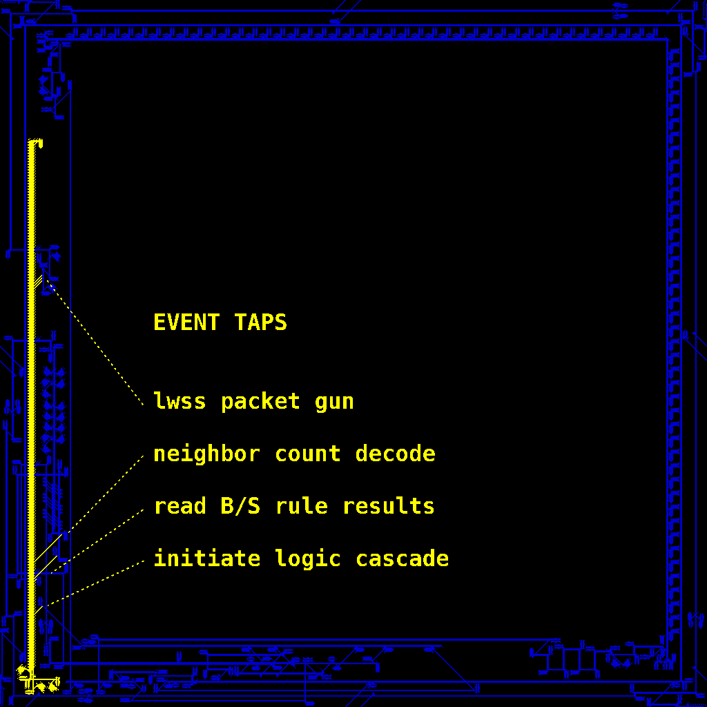
Finally, the block is destroyed at the source of the tractor beam and restored in its starting position, beginning the cycle again.

Encoding the Rules

The rules of the metapixel are encoded in two columns (like hardware registers) as shown in the images below:

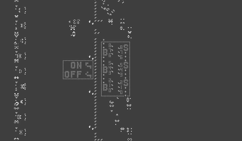
Life-like automata rules are written in the form B#/S#, described here. Conway’s rules are defined as B3/S23, so the corresponding bits of the registers of the OTCA metapixel are populated with one Eater-1 each:

Counting Neighbors

On each clock cycle three sets of three LWSSes (9 total) leave the LWSS packet gun (triggered by the clock, explained above) and complete a loop around the metapixel, passing by each of the metapixel’s Moore neighbors on the way. As the LWSSes pass by each neighbor, the first ship in the train collides with a pond in its path if that neighbor is currently in an “alive” state; this collision destoys the ship and decreases the total number of ships in the train by one. If the neighbor is not alive, then no pond is present and the ships go by unharmed. Since the train starts with 9 LWSSes, if a metapixel has 4 alive neighbors then only five LWSSes will return after completing a pass around the perimeter. A collision of a train of LWSSes with a pond is shown below at about 0:26 (I’ll explain how the ponds get there later):

This video also shows the shepherding of the train of LWSSes around the metapixel by twin bees shuttles and other reflectors, and an example of “color adjustment” of the ships (changing their phase slightly) by a pair of glider guns. The path of the LWSSes and the location of color adjusters and possible ponds is shown in this image.

The full path of the LWSS train is shown below. Notice how one ship is removed from the front of the train as it passes each living neighbor.

Comparing Neighbor Count with Rules

When the train of LWSSes completes a loop, they are channeled into a mechanism (sync buffer and p46 to p40 converter) where they given the same phase. Then they are sent into the rules register where they are collided with another LWSS coming from the opposite direction (originating from one of the gliders shot out of the clock) to decode the train of LWSS into the number of living neighbors (shown in this diagram).

The location of the collision between the LWSS train and the LWSS originating from the clock depends on how many LWSSes were destroyed from the front of the train during the loop around the metapixel. The mechanism is set up so that the collision shoots out two gliders in opposite directions, aimed towards the register that corresponds to the number of living neighbors the metapixel has (again, see this pic as a reference).

Normally, the gliders will each collide with a beehive to produce a block and a pond, this is called a honeybit reaction. If you watch from about 6:00 into the video above, you’ll see the collision of the antiparallel LWSSes, sending two gliders towards 4th slot (count up from the bottom, starting at 0) in both the birth and survival registers, and at about 6:30 two ponds are formed in the registers. The remaining spaceships in the LWSS train collide with an Eater-1 and are destroyed. The video below shows a closer look across many generations:

If the slot in the register is occupied by an Eater-1 (as are the 3rd slot in the birth register, and the 2nd and 3rd slots in the survival registers, again counting up from the bottom starting at 0), then the incoming glider is destroyed before it has a chance to initiate a honeybit reaction with the beehive. This produces no pond in the register. In this mechanism a register has a pond if the number of living neighbors doesn’t satisfy the conditions for life in the next generation, and no pond if it does. Remember this information is split between two registers (birth and survival) and in a later step some logic will look at the current state of the metapixel to determine which register to read from (described later). This mechanism is what makes the OTCA Metapixel programmable for any Life-like ruleset, pretty cool.

Next, the clock shoots out a pair of LWSSes to read these registers (one LWSS for each register), following the trajectories shown in this diagram. If a pond is present in a register, the LWSS collides with the pond and is destroyed. This completes the honeybit reaction and restores the beehive back to its original state. If the LWSS has no pond in its path, it is allowed to continue into the next logic bank. In the video above, see if you can predict the next state of the metapixel by reading from the registers.

Accessing Neighbor State

Before I move to the final logic of the system, let’s look at how the neighbor states are tallied up. This diagram shows the 8 input/ouput channels of each metapixel, each corresponding to one of eight neighbors for a single metapixel. By taking a closer look at one of them, you’ll see another honeybit reaction happening:

The honeybit reaction on the left corresponds to the state of the metapixel on the right, and the reaction on the right corresponds to the state of the metapixel on the left. The LWSS train moves clockwise around the metapixel, so the train moving down the screen belongs to the pixel on the left and the train moving up the screen belongs to the pixel on the right.

These honeybit reactions are set by a middle weight spaceship (MWSS) that moves in a counter-clockwise path around the pixel each clock cycle. Here is a description of its path and the path of all the gliders it generates for 8 honeybit reactions around the metapixel. The MWSS is created only if the current state of the metapixel is alive and at the end of its loop around the pixel it is destroyed.

Determining the Next State

The final state of the system is read from a series of logic gates. As has already been demonstrated in some of the previous sections, logic in Life is typically achieved by sending spaceships (usually gliders) through a path where they may or may not collide with other objects and be annihilated. At the end of their journey, a reading mechanism tests for their presence (1) or absence (0). Here’s a video that shows some concrete examples of various boolean operations. Long “glider tapes” can even be used as persistent memory to store large amounts of information, demonstrated in Gemini and this programmable text generator (the “Golly ticker”).

The final logic of the metapixel is summarized in this diagram.

First some definitions:

C is the current state of the cell, 1 or 0

B is the state of the birth register, 1 for satisfied birth conditions, 0 for not-satisfied

S if the state of the survival register, 1 for satisfied, 0 for not-satisfied

The states of C, B, and S are stored in the metapixel by the presence (“1”) or absence (“0”) of three boats. Boats have the interesting property that when they are hit with a glider they reflect a new glider with a trajectory that is perpendicular to the path of the incoming glider. This collision destroys the boat, so boats are known as one time reflectors. The B and S boats (shown in this diagram) are set using the LWSSes that are able to pass through the birth and survival registers during the decoding step described above. In this video, watch how boats are placed at B and S by a pair of LWSSes starting at 3:47, the moment they are set comes at 4:52:

A glider is used to read the states of C, B, and S and set a pond at G or H (shown in this diagram). The logic for G and H pond formation (“1” means a pond is formed, “0” means no pond) is given by the following logic:

G = C & !S (G equals 1 when C is 1 and S is 0, else G is 0)

H = !C & B (H equals 1 when C is 0 and B is 1, else H is 0)

The final glider released by the clock (described at the beginning) sets off a logic cascade that computes these relationships. The glider is released through the small hole in the fence next to the clock, a little less than halfway up the left side of the video above (15:45), triggering the formation of a LWSS (15:48) which travels toward the right side of the video, releasing two gliders on its way (16:11). The first glider bounces around and eventually turns into a LWSS that reads the results of G and H, more on that in the next paragraph. The second glider heads towards C, if C is present it reflects and starts heading toward S. If S is present it reflects into an eater and dies, if S is not present it continues to a beehive at G and does a honeybit reaction, forming a pond. If C is not present, the second glider heads toward B instead. If B is present, the glider reflects off B and does a honeybit reaction at H, otherwise it runs into an eater and dies. Starting at 16:20 in the video above, we see the glider being created, reflecting off C, passing through an absent S, and finally, forming a pond at G.

At 16:37 you can see a pond set at G and a LWSS coming in from the left to read G and H. If either G or H has a pond set, the LWSS is destroyed, as shown at 16:39. If neither are set (see 10:47) the LWSS continues on and forms a boat at !T (shown as T with a line on top on this diagram). This can be summarized with the logic:

!T = !(G | H) (!T equals 1 when G and H are both 0, else !T is 0)

A third glider released at 10:56 by the original LWSS trigger heads toward !T. If the boat at !T is present the glider reflects off the boat and hits an eater, if the boat is not present it continues to T (again, this diagram). The glider is destroyed by an eater in 11:17, but you can see it turn into a LWSS and head to T during a previous iteration starting at 5:33.

A fourth glider is released by the original LWSS which turns into a LWSS that cleans up any leftover boats left at B or S after the logical operations have completed. An example starts at 5:23. This LWSS has no other function, it is destroyed either by a boat it cleans up, or an eater. Its trajectory is shown here.

After all this we’re left with the following state:

T = presence of a LWSS at T, the formal logic for this state is given by:

T = !(!T) = G | H = (C & !S) | (!C & B)

which you can read as “T is 1 if the pixel is currently alive and it doesn’t satisfy the requirements for survival, or if the pixel is currently dead and does satisfy the requirements for birth, otherwise it is 0” – basically a LWSS at T means the metapixel should toggle its current state.

(just a bit longer, sorry this is kind of a slog)

The LWSS at T follows the path shown here. At 6:28 you can see the LWSS transform into a glider and back again, while navigating through a series of twists and turns. At 6:39 it shoots a glider angled upward which turns into an LWSS that heads to the sync buffer and eventually the cell state boat bit (different than C, more on this in the next paragraph). The original LWSS continues to the left, shooting another two gliders off at 6:42 and 6:48; each of these gliders turns into a LWSS and one heads to the bottom right corner and the other to the top left corner of the metapixel to toggle the state of the output display (more on that in the next section).

The cell state boat bit is what actually stores the current state of the cell, (C is updated periodically based on the state of the boat bit). If the boat bit is present, indicating that the current state of the metapixel is “off”, the incoming LWSS will form a glider that collides with it and removes it (starts at 7:03). If the cell state boat bit is not present, indicating that the current state of the metapixel is “on”, the incoming LWSS will form a glider that creates a new boat bit (starts at 18:58).

Finally, let’s follow the path of the original LWSS that triggered this whole series of events. It follows the outer path shown here, gets converted into a MWSS and heads towards the cell state boat bit. If the boat bit is present it collides with it and dies, though it does preserve the boat bit during this death (3:18). If the boat bit is not present it passes by unharmed and keeps heading to the right (7:14). This is the same MWSS that does a counterclockwise loop around the cell, triggering honeybit reactions on all the neighbors’ inputs. This MWSS is only allowed to do the loop when the cell state boat bit is not present, when the metapixel is “on”. Just before it leaves to do the loop it shoots off a glider that bounces around and eventually sets a boat at C (7:18). At 7:53 you can see it setting off the first of 8 honeybit reactions around the metapixel, one for each Moore neighbor.

Output Display

The last piece of the metapixel is the output display that uses a ton of spaceships to fill in a big square area so it looks more or less white. Two synchronized LWSSes toggle the output display; they came from the logic mechanism described in the previous paragraphs, shown here. Their timing is synced up through a series of bends in their path and glider transformations, then they are used to toggle a HWSS gun that triggers a series of LWSS “out of the blue” reactions. The streams of LWSSes fill the square space and mutually annihilate each other in the center of the metapixel, shown here. The mechanisms for both latches are similar: